Linear regression strives to show the relationship between two variables by applying a linear equation to observed data. One variable is supposed to be an independent variable, and the other is to be a dependent variable. For example, the weight of the person is linearly related to his height. Hence this shows a linear relationship between the height and weight of the person. As the height is increased, the weight of the person also gets increased.

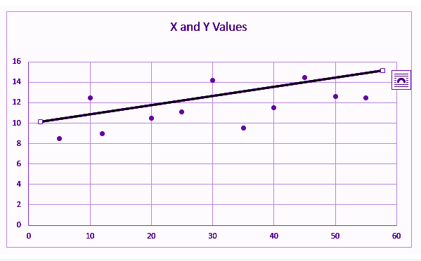
It is not necessary that here one variable is dependent on others, or one causes the other, but there is some critical relationship between the two variables. In such cases, we use a scatter plot to imply the strength of the relationship between the variables. If there is no relation or linking between the variables, the scatter plot does not indicate any increasing or decreasing pattern. For such cases, the linear regression design is not beneficial to the given data.

Also, read:

Linear Regression Equation

The measure of the extent of the relationship between two variables is shown by the correlation coefficient. The range of this coefficient lies between -1 to +1. This coefficient shows the strength of the association of the observed data for two variables.

A linear regression line equation is written in the form of:

Y = a + bX

where X is the independent variable and plotted along the x-axis

Y is the dependent variable and plotted along the y-axis

The slope of the line is b, and a is the intercept (the value of y when x = 0).

Linear Regression Formula

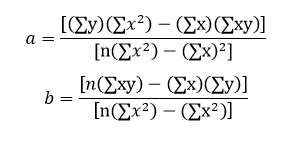
Linear regression shows the linear relationship between two variables. The equation of linear regression is similar to the slope formula what we have learned before in earlier classes such as linear equations in two variables. It is given by;

Y= a + bX

Now, here we need to find the value of the slope of the line, b, plotted in scatter plot and the intercept, a.

Simple Linear Regression

The very most straightforward case of a single scalar predictor variable x and a single scalar response variable y is known as simple linear regression. The equation for this regression is represented by;

y=a+bx

The expansion to multiple and vector-valued predictor variables is known as multiple linear regression, also known as multivariable linear regression. The equation for this regression is represented by;

Y = a+bX

Almost all real-world regression patterns include multiple predictors, and basic explanations of linear regression are often explained in terms of the multiple regression form. Note that, though, in these cases, the dependent variable y is yet a scalar.

Least Square Regression Line or Linear Regression Line

The most popular method to fit a regression line in the XY plot is the method of least-squares. This process determines the best-fitting line for the noted data by reducing the sum of the squares of the vertical deviations from each data point to the line. If a point rests on the fitted line accurately, then its perpendicular deviation is 0. Because the variations are first squared, then added, their positive and negative values will not be cancelled.

Linear regression determines the straight line, called the least-squares regression line or LSRL, that best expresses observations in a bivariate analysis of data set. Suppose Y is a dependent variable, and X is an independent variable, then the population regression line is given by;

Y = B₀+B₁X

Where

B₀ is a constant

B₁ is the regression coefficient

If a random sample of observations is given, then the regression line is expressed by;

ŷ = b₀ + b₁x

where b₀ is a constant, b₁ is the regression coefficient, x is the independent variable, and ŷ is the predicted value of the dependent variable.

Properties of Linear Regression

For the regression line where the regression parameters b₀ and b₁ are defined, the properties are given as:

• The line reduces the sum of squared differences between observed values and predicted values.
• The regression line passes through the mean of X and Y variable values
• The regression constant (b₀) is equal to y-intercept the linear regression
• The regression coefficient (b₁) is the slope of the regression line which is equal to the average change in the dependent variable (Y) for a unit change in the independent variable (X).

Regression Coefficient

In the linear regression line, we have seen the equation is given by;

Y = B₀+B₁X

Where

B₀ is a constant

B₁ is the regression coefficient

Now, let us see the formula to find the value of the regression coefficient.

B₁ = b₁ = Σ [ (x_i – x)(y_i – y) ] / Σ [ (x_i – x)²]

Where x_i and y_i are the observed data sets.

And x and y are the mean value.