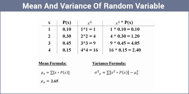
Mean And Variance Of Random Variable
Probability distribution of a random variable is defined as a description accounting the values of the random variable along with the corresponding probabilities. In many cases we express the feature of random variable with the help of a single value computed from its probability distribution. These values can either be mean or median or mode.

Mean of random variable
Let \(X\) be a random variable with possible values \(x_1, x_2, x_3, … , x_n\) occurring with probabilities \(p_1, p_2, p_3, … ,p_n\), respectively. The mean of a random variable \(X\), denoted by \(μ\), is the weighted average of the possible values of \(X\), each value being weighted by its probability of occurrence. The mean of a random variable X is also knows as expectation of \(X\) given by,
\(E(X)~=~ μ~=~\sum\limits_{i=1}^{n}~x_i p_i\)
=\(x_1 p_1~+~x_2 p_2~+~⋯~+~x_n p_n\)
Example
Illustration 1: Calculate the mean of the number obtained on rolling an unbiased die.
Solution: The sample space of the experiment, \(S\) = {1, 2, 3, 4, 5, 6}.
Let the number obtained after rolling the die be \(X\). Basically, \(X\) is a random variable which can take any value from 1, 2, 3, 4, 5 and 6.
If \( P(1)\) represents probability of getting 1 after rolling the die, then
\(P(1)~ =~ P(2)~ =~ P(3)~ = ~P(4)~ = ~P(5)~ = ~P(6)~ = ~\frac{1}{6}\)
Probability distribution of X can be given as,
| X | 1 | 2 | 3 | 4 | 5 | 6 |
| P(X) | \(\frac{1}{6}\) | \(\frac{1}{6}\) | \(\frac{1}{6}\) | \(\frac{1}{6}\) | \(\frac{1}{6}\) | \(\frac{1}{6}\) |
\(E(X)~=~ μ~=~\sum\limits_{i=1}^{n}x_i p_i\)
\(\sum\limits_{i=1}^{6}~x_i p_i~=~1. \frac{1}{6}~+~2.\frac{1}{6}~+~3.\frac{1}{6}~+~4.\frac{1}{6}~+~5.\frac{1}{6}~+~6.\frac{1}{6}\)
=\(\frac{1}{6}~+~\frac{2}{6}~+~\frac{3}{6}~+~\frac{4}{6}~+~\frac{5}{6}~+~\frac{6}{6}~=~\frac{21}{6}~=~3.5\)
There is an important point to note here. If each of the values of a random variable (\(a_1,a_2,…,a_n\)) has equal probability of occurring (\(\frac{1}{n}\)), then mean is given by \(\left(\frac{a_1+ a_2+⋯+a_n}{n}\right)\).
Mean of random variables with different probability distributions can have same values. Hence, mean fails to explain the variability of values in probability distribution. Therefore, variance of random variable is defined to measure the spread and scatter in data. Variance of a random variable is discussed in detail here on.
Variance of random variable
Basically, the variance tells us how spread-out the values of X are around the mean value. Variance of a random variable (denoted by \(σ_x^2\)) with values \(x_1, x_2, x_3, … , x_n\) occurring with probabilities \(p_1, p_2, p_3,…, p_n\) can be given as :
\(Var(X)~=~σ_x^2~=~\sum\limits_{i=1}^n(x_i~-~μ)^2 p_i\)
\(Var(X)~=~\sum\limits_{i=1}^n~(x_i)^2 p_i~+~\sum\limits_{i=1}^n~μ^2 p_i~-~\sum\limits_{i=1}^n~2x_{i} μp_i\)
\(Var(X)~=~\sum\limits_{i=1}^n~(x_i)^2 p_i~+~μ^2~\sum\limits~_{i=1}^n~p_i~ -~2μ\sum\limits_{i=1}^n~x_{i} p_i\)
Here,
\(\sum\limits_{i=1}^{n}x_{i}p_{i}~= ~μ\) (Mean of \(X\)) and \(\sum\limits_{i=1}^{n}~p_{i}~=~1\) (sum of probabilities of all the outcomes of an event is 1). Substituting the values, we get
\(Var(X)~=~\sum\limits_{i=1}^{n}(x_i)^2 p_i ~+~ μ^2~-~ 2μ^2\)
\(σ_x^2~=~ Var(X)~=~\sum\limits_{i=1}^{n}~(x_i)^2 p_i~- ~μ^2\)
\(Var(X)~ =~ E(X^2)~ – ~[E(X)]^2\)
Where,
\(E(X^2)~=~\sum\limits_{i=1}^{n}(x_i)^2 p_i\) and \(E(X)~=~\sum\limits_{i=1}^{n}x_{i}p_i\)
An illustration of application of the concept is given below.
Example
Illustration 2: Two cards are drawn successively with replacement from a well shuffled pack of 52 cards. Find the mean and variance of the number of aces.
Solution: Let \(X\) be a random variable denoting the number of aces. Possible values of \(X\) are 0, 1,2.
\(P(X ~=~ 0)~ = ~P(non-ace~ and ~non-ace)\)
=\( P(non-ace)~ × ~P(non-ace)\)
= \(\frac{48}{52}~×~\frac{48}{52} ~= ~\frac{144}{169}\)
\(P(X ~=~ 1)~ =~ P(ace~ and~ non-ace~ or~ non-ace~ and~ ace)\)
= \(P(ace~ and ~non-ace) ~+~ P(non-ace~ and~ ace)\)
= \(P(ace) ~×~ P(non-ace) ~+~ P ~(non-ace) ~× ~P(ace)\)
= \(\frac{4}{52}~×~\frac{48}{52}~+~\frac{48}{52}~×~\frac{4}{52}~=~\frac{24}{169}\)
\(P(X~ =~ 2)~ = ~P ~(ace~ and~ ace)\)
= \(P(ace)~ × ~P(ace)\)
=\(\frac{4}{52}~×~\frac{4}{52} ~=~ \frac{1}{169}\)
Thus, the probability distribution can be given as,
| X | 0 | 1 | 2 |
| P(X) | \(\frac{144}{169}\) | \(\frac{24}{169}\) | \(\frac{1}{169}\) |
\(E(X)~=~ μ~=~\sum\limits_{i=1}^{n}x_i p_i ~=~\frac{0.144}{169}~+~1.\frac{24}{169}~+~2.\frac{1}{169}\)
=\(0~+~\frac{24}{169}~+~\frac{2}{169}~=~\frac{26}{169}\)
\(E(X^2)~=~\sum\limits_{i=1}^{n}~(x_i)^2 p_i~=~ 0^2.\frac{144}{169}~+~1^2.\frac{24}{169}~+~2^2.\frac{1}{169}\)
=\(0~+~\frac{24}{169}~+~\frac{4}{169}~=~\frac{28}{169}\)
\(Var(X)~ = ~E(X^2)~ – ~[E(X)]^2~ = ~\frac{28}{169}~-~(\frac{26}{169})^2~=~\frac{24}{169}\)<
For detailed discussion on the probability distribution of random variables, download Byju’s-the learning app.
‘