We have already seen that two matrices are equal when they are of the same order and their corresponding elements are equal. That is, if \(P\) = \([p_{ij}]_{m×n}\) and \(Q\) = \( [q_{ij}]_{r×s}\) are two matrices such that \(P\) = \( Q\), then:

 

• \( m \) =\( r \) and \( n \) = \( s \) i.e. the orders of the two matrices must be same
• For every value of i and j, \(p_{ij}\) = \( q_{ij}\).

But there is another way to compare matrices. In this case, the matrices are equivalent to each other. For a matrix  \( P \) = \([p_{ij}]_{m×n}\) to be equivalent to a matrix \(Q\) = \([q_{ij}]_{r×s}\), i.e. P ~ Q , the following two conditions must be satisfied:

• m = r and n = s; again, the orders of the two matrices must be the same

• P should get transformed to Q using the elementary transformation and vice-versa.

Elementary transformation of matrices is very important. It is used to find equivalent matrices and also to find the inverse of a matrix. Elementary transformation is playing with the rows and columns of a matrix. Let us learn how to perform the transformation on matrices.

Elementary Row Transformation

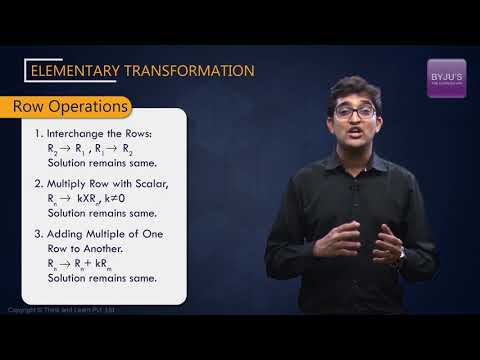
As the name suggests, only the rows of the matrices are transformed and NO changes are made in the columns. These row operations are executed according to a certain set of rules which make sure that the transformed matrix is equivalent to the original matrix. These rules are:

• Any two rows are interchangeable. The interchange of \(i^{th}\) and \(j^{th}\) rows is represented as:

\(R_i ↔ R_j \)

For example: If \(A\) = \(\begin{bmatrix}
1 & 23\cr
-9 & 5\cr
-13 & 7
\end{bmatrix}\), applying \(R_1 ↔ R_3\), we get \( B\) =\(\begin{bmatrix}
-13 & 7\cr
-9 & 5\cr
1 & 23
\end{bmatrix}\). Here, A ~ B.

• All the elements of any row can be multiplied to any non-zero number. The multiplication of \( i^{th} \) row to a non-zero number k, is represented as:

\(R_i \rightarrow kR_i\)

For example: If A = \(\begin{bmatrix}
1 & 6 & 8\cr
3 & 5 & 21\cr
2 & 1 & 9
\end{bmatrix}\), applying \(R_2 \rightarrow 2R_2\), we get \(B \)= \(\begin{bmatrix}
1 & 6 & 8\cr
6 & 10 & 42\cr
2 & 1 & 9
\end{bmatrix}\). Again, A ~ B.

• All the elements of a row can be added to corresponding elements of another row multiplied by any non-zero constant. If the elements of \( i^{th} \) row are being added to the elements of \( j^{th} \) row (multiplied by a non-zero number k), then it is represented as:

\( R_i \rightarrow R_i + k R_j \)

An important thing to note here is that the change will only reflect in the elements of \( i^{th} \) row. The elements of \( j^{th} \) row will remain same.

For example: If \(  A \)=\(\begin{bmatrix}4 & 10 & 64\cr   1 & -13 & 9\cr
2 & 5 & 32  \end{bmatrix}\), applying \(R_1 \rightarrow R_1 + (-2)R_3\) , we get\( B\) = \(\begin{bmatrix} 0 & 0 & 0\cr    1 & -13 & 9\cr
2 & 5 & 32   \end{bmatrix}\). Here,  A ~ B .

It’s easy to figure out here that if k = 1, it just reduces to adding the elements of \(i^{th}\) row to corresponding elements of \(j^{th}\) row. Also, if k = -1, it means subtracting the elements of \(j^{th}\) row from corresponding elements of the \(i^{th}\) row.

For example: If \( P \) = \(\begin{bmatrix}1 & 5 & 4\cr    5 & 2 & 5\cr    4 & 5 & 3 \end{bmatrix} \), applying \(R_2 \rightarrow R_2 + R_3 \), we get \(Q \) = \(\begin{bmatrix} 1 & 5 & 4\cr 9 & 7 & 8\cr  4 & 5 & 3
\end{bmatrix}\). P ~ Q

Those were the three elementary row transformations/operations. The elementary column operations are exactly the same operations done on the columns.

Elementary Column Operation

Those three operations for rows, if applied to columns in the same way, we get elementary column operation. As we have already discussed row transformation in detail, we will briefly discuss column transformation. The rules for elementary column transformation are:

• Any two columns are interchangeable i.e.\( C_i ↔ C_j\) .

For example: If \(A \)=\(\begin{bmatrix}
1 & 23\cr
-9 & 5 \cr
-13 & 7
\end{bmatrix}
\), applying \(C_1 ↔ C_2 \), we get \(B\) =\(\begin{bmatrix}
23 & 1\cr
5 & -9\cr
7 & -13
\end{bmatrix}\)

Here,  A ~ B . 

• All the elements of any column can be multiplied to any non-zero number i.e.\( C_i ↔ k C_i\).

For example: If \(A\) =
\(\begin{bmatrix}
1 & 6 & 8\cr
3 & 5 & 21\cr
2 & 1 & 9
\end{bmatrix}\), applying \(C_2 \rightarrow 3 C_2\), we get \(B\) =\(\begin{bmatrix}
1 & 18 & 8 \cr
3 & 15 & 21\cr
2 & 3 & 9
\end{bmatrix}\)
. Again,  A ~ B .

• All the elements of a column can be added to corresponding elements of another column multiplied by any non-zero constant i.e. \(C_i \rightarrow C_i + k C_j \)

For example: If \(A\) = \(\begin{bmatrix}
4 & 10 & 1\cr
1 & -13 & 1\cr
2 & 5 & 2
\end{bmatrix}\), applying \(C_1 \rightarrow C_1 + 3C_3\), we get \(B\) = \( \begin{bmatrix}
7 & 10 & 1\cr
4 & -13 & 1\cr
8 & 5 & 2
\end{bmatrix}\).. Here,  A ~ B .

Those were the elementary transformation techniques for matrices. As mentioned before, these are very important and are used to find the inverse of a matrix. To know how to find the inverse of a matrix, visit www.byjus.com and learn the concepts, explained in a very easy way.