Exponential Smoothing
Exponential smoothing was first suggested in the statistical literature without reference to previous work by Robert Goodell Brown in 1956 and then expanded by Charles C. Holt in 1957. Exponential smoothing is a broadly accurate principle for smoothing time series data using the exponential window function. The controlling input of the exponential smoothing calculation is defined as the smoothing factor or the smoothing constant.
As we know that, in the simple moving average, the past observations are weighted equally, exponential functions are used to assign exponentially decreasing weights over time. It is an easily learned and easily applied method for making some determination based on prior assumptions by the user, such as seasonality. Exponential smoothing is generally used for the analysis of time-series data.
Exponential Smoothing Formula
The simplest form of an exponential smoothing formula is given by:
st = αxt+(1 – α)st-1= st-1+ α(xt – st-1)
Here,
st = smoothed statistic, it is the simple weighted average of current observation xt
st-1 = previous smoothed statistic
α = smoothing factor of data; 0 < α < 1
t = time period
If the value of the smoothing factor is larger, then the level of smoothing will reduce. Value of α close to 1 has less of a smoothing effect and give greater weight to recent changes in the data, while the value of α closer to zero has a greater smoothing effect and are less responsive to recent changes.
There is no official accurate procedure for choosing α. The statistician’s judgment is used to choose an appropriate factor sometimes. Otherwise, a statistical technique may be used to optimize the value of α. For example, the method of least squares can be used to determine the value of α for which the sum of the quantities is minimized.
Exponential Smoothing Forecasting
Exponential smoothing is generally used to make short term forecasts, but longer-term forecasts using this technique can be quite unreliable. More recent observations given larger weights by exponential smoothing methods, and the weights decrease exponentially as the observations become more distant. When the parameters describing the time series are changing slowly over time, then these methods are most effective.
Exponential Smoothing Methods
There are three main methods to estimate exponential smoothing. They are:
- Simple or single exponential smoothing
- Double exponential smoothing
- Triple exponential smoothing
Simple or single exponential smoothing
If the data has no trend and no seasonal pattern, then this method of forecasting the time series is essentially used. This method uses weighted moving averages with exponentially decreasing weights.
The single exponential smoothing formula is given by:
st = αxt+(1 – α)st-1 = st-1 + α(xt – st-1)
Double exponential smoothing
This method is also called as Holt’s trend corrected or second-order exponential smoothing. This method is used for forecasting the time series when the data has a linear trend and no seasonal pattern. The primary idea behind double exponential smoothing is to introduce a term to take into account the possibility of a series showing some form of trend. This slope component is itself updated through exponential smoothing.
The double exponential smoothing formulas are given by:
S1 = x1
B1 = x1-x0
For t>1,
st = αxt + (1 – α)(st-1 + bt-1)
βt = β(st – st-1) + (1 – β)bt-1
Here,
st = smoothed statistic, it is the simple weighted average of current observation xt
st-1 = previous smoothed statistic
α = smoothing factor of data; 0 < α < 1
t = time period
bt = best estimate of trend at time t
β = trend smoothing factor; 0 < β <1
Triple exponential smoothing
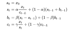
In this method, exponential smoothing applied three times. This method is used for forecasting the time series when the data has both linear trend and seasonal pattern. This method is also called Holt-Winters exponential smoothing.
The triple exponential smoothing formulas are given by:

Here,
st = smoothed statistic, it is the simple weighted average of current observation xt
st-1 = previous smoothed statistic
α = smoothing factor of data; 0 < α < 1
t = time period
bt = best estimate of a trend at time t
β = trend smoothing factor; 0 < β <1
ct = sequence of seasonal correction factor at time t
γ = seasonal change smoothing factor; 0 < γ < 1
Example problem
The sales of a magazine in a stall for the previous 10 months are given below.
| Month | Sales |
| January | 30 |
| February | 25 |
| March | 35 |
| April | 25 |
| May | 20 |
| June | 30 |
| July | 35 |
| August | 40 |
| September | 30 |
| October | 45 |
Calculate the simple exponential smoothing taking α =0.3 for the above data.
Solution:
| Month | Sales | Exponential smooth
α =0.3 |
| January | 30 | 30.00 |
| February | 25 | 30.00 |
| March | 35 | 28.50 |
| April | 25 | 30.45 |
| May | 20 | 14.1 |
| June | 30 | 15.87 |
| July | 35 | 20.109 |
| August | 40 | 24.5763 |
| September | 30 | 29.20341 |
| October | 45 | 29.442387 |
| November | – | 34.1096709 |
Read more: