
Chi-Square Test
A chi-squared test (symbolically represented as χ2) is basically a data analysis on the basis of observations of a random set of variables. Usually, it is a comparison of two statistical data sets. This test was introduced by Karl Pearson in 1900 for categorical data analysis and distribution. So it was mentioned as Pearson’s chi-squared test.
The chi-square test is used to estimate how likely the observations that are made would be, by considering the assumption of the null hypothesis as true.
A hypothesis is a consideration that a given condition or statement might be true, which we can test afterwards. Chi-squared tests are usually created from a sum of squared falsities or errors over the sample variance.
| Table of contents: |
Chi-Square Distribution
When we consider, the null speculation is true, the sampling distribution of the test statistic is called as chi-squared distribution. The chi-squared test helps to determine whether there is a notable difference between the normal frequencies and the observed frequencies in one or more classes or categories. It gives the probability of independent variables.
Note: Chi-squared test is applicable only for categorical data, such as men and women falling under the categories of Gender, Age, Height, etc.
Finding P-Value
P stands for probability here. To calculate the p-value, the chi-square test is used in statistics. The different values of p indicates the different hypothesis interpretation, are given below:
- P≤ 0.05; Hypothesis rejected
- P>.05; Hypothesis Accepted
Probability is all about chance or risk or uncertainty. It is the possibility of the outcome of the sample or the occurrence of an event. But when we talk about statistics, it is more about how we handle various data using different techniques. It helps to represent complicated data or bulk data in a very easy and understandable way. It describes the collection, analysis, interpretation, presentation, and organization of data. The concept of both probability and statistics is related to the chi-squared test.
Also, read:
Properties
The following are the important properties of the chi-square test:
- Two times the number of degrees of freedom is equal to the variance.
- The number of degree of freedom is equal to the mean distribution
- The chi-square distribution curve approaches the normal distribution when the degree of freedom increases.
Formula
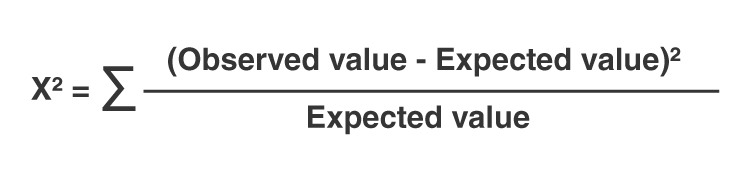
The chi-squared test is done to check if there is any difference between the observed value and expected value. The formula for chi-square can be written as;
or
χ2 = ∑(Oi – Ei)2/Ei
where Oi is the observed value and Ei is the expected value.
Chi-Square Test of Independence
The chi-square test of independence also known as the chi-square test of association which is used to determine the association between the categorical variables. It is considered as a non-parametric test. It is mostly used to test statistical independence.
The chi-square test of independence is not appropriate when the categorical variables represent the pre-test and post-test observations. For this test, the data must meet the following requirements:
- Two categorical variables
- Relatively large sample size
- Categories of variables (two or more)
- Independence of observations
Example of Categorical Data
Let us take an example of a categorical data where there is a society of 1000 residents with four neighbourhoods, P, Q, R and S. A random sample of 650 residents of the society is taken whose occupations are doctors, engineers and teachers. The null hypothesis is that each person’s neighbourhood of residency is independent of the person’s professional division. The data are categorised as:
| Categories | P | Q | R | S | Total |
| Doctors | 90 | 60 | 104 | 95 | 349 |
| Engineers | 30 | 50 | 51 | 20 | 151 |
| Teachers | 30 | 40 | 45 | 35 | 150 |
| Total | 150 | 150 | 200 | 150 | 650 |
Assume the sample living in neighbourhood P, 150, to estimate what proportion of the whole 1,000 people live in neighbourhood P. In the same way, we take 349/650 to calculate what ratio of the 1,000 are doctors. By the supposition of independence under the hypothesis, we should “expect” the number of doctors in neighbourhood P is;
150 x 349/650 ≈ 80.54
So by the chi-square test formula for that particular cell in the table, we get;
(Observed – Expected)2/Expected Value = (90-80.54)2/80.54 ≈ 1.11
Some of the exciting facts about the Chi-square test are given below:
The Chi-square statistic can only be used on numbers. We cannot use them for data in terms of percentages, proportions, means or similar statistical contents. Suppose, if we have 20% of 400 people, we need to convert it to a number, i.e. 80, before running a test statistic.
A chi-square test will give us a p-value. The p-value will tell us whether our test results are significant or not.
However, to perform a chi-square test and get the p-value, we require two pieces of information:
(1) Degrees of freedom. That’s just the number of categories minus 1.
(2) The alpha level(α). You or the researcher chooses this. The usual alpha level is 0.05 (5%), but you could also have other levels like 0.01 or 0.10.
In elementary statistics, we usually get questions along with the degrees of freedom(DF) and the alpha level. Thus, we don’t usually have to figure out what they are. To get the degrees of freedom, count the categories and subtract 1.
Table
The chi-square distribution table with three probability levels is provided here. The statistic here is used to examine whether distributions of certain variables vary from one another. The categorical variable will produce data in the categories and numerical variables will produce data in numerical form.
The distribution of χ2 with (r-1)(c-1) degrees of freedom(DF), is represented in the table given below. Here, r represents the number of rows in the two-way table and c represents the number of columns.
| DF |
Value of P |
||
| 0.05 | 0.01 | 0.001 | |
| 1 | 3.84 | 6.64 | 10.83 |
| 2 | 5.99 | 9.21 | 13.82 |
| 3 | 7.82 | 11.35 | 16.27 |
| 4 | 9.49 | 13.28 | 18.47 |
| 5 | 11.07 | 15.09 | 20.52 |
| 6 | 12.59 | 16.81 | 22.46 |
| 7 | 14.07 | 18.48 | 24.32 |
| 8 | 15.51 | 20.09 | 26.13 |
| 9 | 16.92 | 21.67 | 27.88 |
| 10 | 18.31 | 23.21 | 29.59 |
| 11 | 19.68 | 24.73 | 31.26 |
| 12 | 21.03 | 26.22 | 32.91 |
| 13 | 22.36 | 27.69 | 34.53 |
| 14 | 23.69 | 29.14 | 36.12 |
| 15 | 25.00 | 30.58 | 37.70 |
| 16 | 26.30 | 32.00 | 39.25 |
| 17 | 27.59 | 33.41 | 40.79 |
| 18 | 28.87 | 34.81 | 42.31 |
| 19 | 30.14 | 36.19 | 43.82 |
| 20 | 31.41 | 37.57 | 45.32 |
| 21 | 32.67 | 38.93 | 46.80 |
| 22 | 33.92 | 40.29 | 48.27 |
| 23 | 35.17 | 41.64 | 49.73 |
| 24 | 36.42 | 42.98 | 51.18 |
| 25 | 37.65 | 44.31 | 52.62 |
| 26 | 38.89 | 45.64 | 54.05 |
| 27 | 40.11 | 46.96 | 55.48 |
| 28 | 41.34 | 48.28 | 56.89 |
| 29 | 42.56 | 49.59 | 58.30 |
| 30 | 43.77 | 50.89 | 59.70 |
| 31 | 44.99 | 52.19 | 61.10 |
| 32 | 46.19 | 53.49 | 62.49 |
| 33 | 47.40 | 54.78 | 63.87 |
| 34 | 48.60 | 56.06 | 65.25 |
| 35 | 49.80 | 57.34 | 66.62 |
| 36 | 51.00 | 58.62 | 67.99 |
| 37 | 52.19 | 59.89 | 69.35 |
| 38 | 53.38 | 61.16 | 70.71 |
| 39 | 54.57 | 62.43 | 72.06 |
| 40 | 55.76 | 63.69 | 73.41 |
| 41 | 56.94 | 64.95 | 74.75 |
| 42 | 58.12 | 66.21 | 76.09 |
| 43 | 59.30 | 67.46 | 77.42 |
| 44 | 60.48 | 68.71 | 78.75 |
| 45 | 61.66 | 69.96 | 80.08 |
| 46 | 62.83 | 71.20 | 81.40 |
| 47 | 64.00 | 72.44 | 82.72 |
| 48 | 65.17 | 73.68 | 84.03 |
| 49 | 66.34 | 74.92 | 85.35 |
| 50 | 67.51 | 76.15 | 86.66 |
| 51 | 68.67 | 77.39 | 87.97 |
| 52 | 69.83 | 78.62 | 89.27 |
| 53 | 70.99 | 79.84 | 90.57 |
| 54 | 72.15 | 81.07 | 91.88 |
| 55 | 73.31 | 82.29 | 93.17 |
| 56 | 74.47 | 83.52 | 94.47 |
| 57 | 75.62 | 84.73 | 95.75 |
| 58 | 76.78 | 85.95 | 97.03 |
| 59 | 77.93 | 87.17 | 98.34 |
| 60 | 79.08 | 88.38 | 99.62 |
| 61 | 80.23 | 89.59 | 100.88 |
| 62 | 81.38 | 90.80 | 102.15 |
| 63 | 82.53 | 92.01 | 103.46 |
| 64 | 83.68 | 93.22 | 104.72 |
| 65 | 84.82 | 94.42 | 105.97 |
| 66 | 85.97 | 95.63 | 107.26 |
| 67 | 87.11 | 96.83 | 108.54 |
| 68 | 88.25 | 98.03 | 109.79 |
| 69 | 89.39 | 99.23 | 111.06 |
| 70 | 90.53 | 100.42 | 112.31 |
| 71 | 91.67 | 101.62 | 113.56 |
| 72 | 92.81 | 102.82 | 114.84 |
| 73 | 93.95 | 104.01 | 116.08 |
| 74 | 95.08 | 105.20 | 117.35 |
| 75 | 96.22 | 106.39 | 118.60 |
| 76 | 97.35 | 107.58 | 119.85 |
| 77 | 98.49 | 108.77 | 121.11 |
| 78 | 99.62 | 109.96 | 122.36 |
| 79 | 100.75 | 111.15 | 123.60 |
| 80 | 101.88 | 112.33 | 124.84 |
| 81 | 103.01 | 113.51 | 126.09 |
| 82 | 104.14 | 114.70 | 127.33 |
| 83 | 105.27 | 115.88 | 128.57 |
| 84 | 106.40 | 117.06 | 129.80 |
| 85 | 107.52 | 118.24 | 131.04 |
| 86 | 108.65 | 119.41 | 132.28 |
| 87 | 109.77 | 120.59 | 133.51 |
| 88 | 110.90 | 121.77 | 134.74 |
| 89 | 112.02 | 122.94 | 135.96 |
| 90 | 113.15 | 124.12 | 137.19 |
| 91 | 114.27 | 125.29 | 138.45 |
| 92 | 115.39 | 126.46 | 139.66 |
| 93 | 116.51 | 127.63 | 140.90 |
| 94 | 117.63 | 128.80 | 142.12 |
| 95 | 118.75 | 129.97 | 143.32 |
| 96 | 119.87 | 131.14 | 144.55 |
| 97 | 120.99 | 132.31 | 145.78 |
| 98 | 122.11 | 133.47 | 146.99 |
| 99 | 123.23 | 134.64 | 148.21 |
| 100 | 124.34 | 135.81 | 149.48 |
Solved Problem
Question:
A survey on cars had conducted in 2011 and determined that 60% of car owners have only one car, 28% have two cars, and 12% have three or more. Supposing that you have decided to conduct your own survey and have collected the data below, determine whether your data supports the results of the study.
Use a significance level of 0.05. Also, given that, out of 129 car owners, 73 had one car and 38 had two cars.
Solution:
Let us state the null and alternative hypotheses.
H0: The proportion of car owners with one, two or three cars is 0.60, 0.28 and 0.12 respectively.
H1: The proportion of car owners with one, two or three cars does not match the proposed model.
A Chi-Square goodness of fit test is appropriate because we are examining the distribution of a single categorical variable.
Let’s tabulate the given information and calculate the required values.
| Observed (Oi) | Expected (Ei) | Oi – Ei | (Oi – Ei)2 | (Oi – Ei)2/Ei | |
| One car | 73 | 0.60 × 129 = 77.4 | -4.4 | 19.36 | 0.2501 |
| Two cars | 38 | 0.28 × 129 = 36.1 | 1.9 | 3.61 | 0.1 |
| Three or more cars | 18 | 0.12 × 129 = 15.5 | 2.5 | 6.25 | 0.4032 |
| Total | 129 | 0.7533 |
Therefore, χ2 = ∑(Oi – Ei)2/Ei = 0.7533
Let’s compare it to the chi-square value for the significance level 0.05.
The degrees for freedom = 3 – 1 = 2
Using the table, the critical value for a 0.05 significance level with df = 2 is 5.99.
That means that 95 times out of 100, a survey that agrees with a sample will have a χ2 value of 5.99 or less.
The Chi-square statistic is only 0.7533, so we will accept the null hypothesis.
Learn more statistical concepts with us and download BYJU’S-The Learning App to get personalized Videos.
Frequently Asked Questions – FAQs
What is the chi-square test write its formula?
χ^2 = ∑(O_i – E_i)^2/E_i
Here,
O_i = Observed value
E_i = Expected value
How do you calculate chi squared?
χ^2 = ∑(O_i – E_i)^2/E_i
This can be done as follows.
For each observed number in the data, subtract the corresponding expected value, i.e. (O — E).
Square the difference, (O — E)^2
Divide these squares by the expected value of each observation, i.e. [(O – E)^2 / E].
Finally, take the sum of these values.
Thus, the obtained value will be the chi-squared statistic.